
Author: Phosphen
Compilation: Gans Gans, Bagel Market Prediction Observation
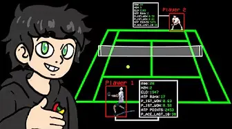
This man collected data from all professional tennis matches over the past 43 years, input it into a machine learning model, and asked only one question: Can you predict who will win?
The model answered with a single word: Yes.
Then, at this year’s Australian Open, it correctly predicted 99 out of 116 matches, with an accuracy of 85%!
This included matches the model had never seen during training, and it even predicted every match of the eventual champion correctly.
All of this was achieved using just a laptop, free data, and open-source code, created by @theGreenCoding.
Next, I will thoroughly break down this goldmine project—from raw data to final successful predictions. This will be the most impressive AI + prediction success story you’ve ever seen.
Starting Point: 43 Years of Tennis Data in a Folder
The story begins with a dataset often called the “Sports Data Holy Grail.”
This dataset covers every professional ATP (Men’s Tennis Association) match from 1985 to 2024.
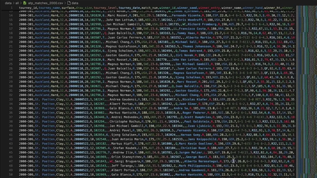
Break points, double faults, forehands, backhands, player heights, ages, rankings, head-to-head records, court surfaces… ATP has tracked every point in detail.
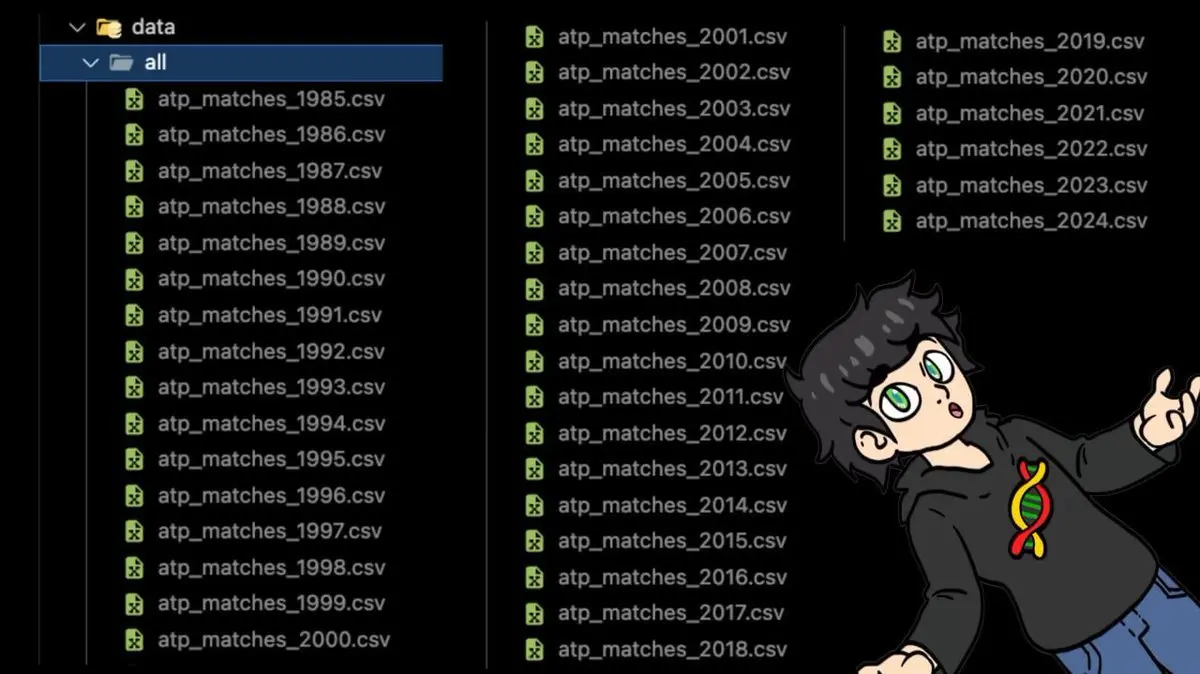
Forty years of CSV files, all stored in one folder.
When he opened the complete dataset, his computer crashed instantly.
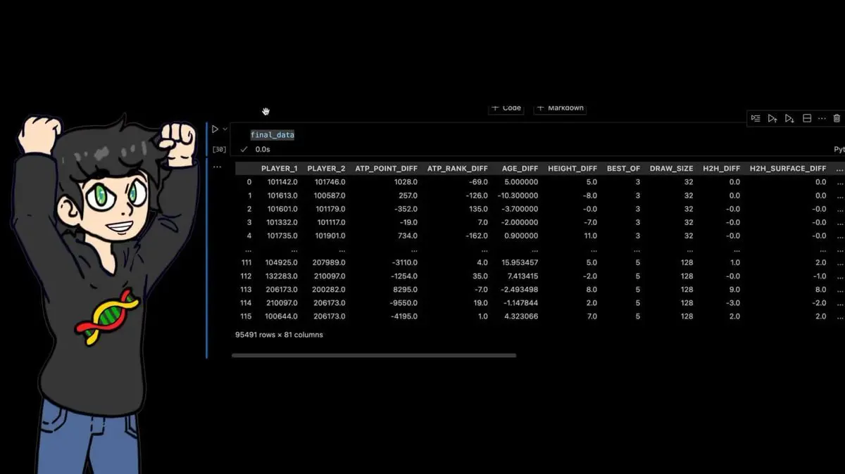
But he didn’t give up. For the 95,491 matches in the dataset, he calculated numerous derived features:
- Head-to-head records between players
- Age difference, height difference
- Win rates over the last 10, 25, 50, 100 matches
- Difference in first serve points won
- Difference in break point save rate
- A custom ELO rating system borrowed from chess (key point)
Final dataset: 95,491 rows × 81 columns.
Every professional tennis match over the past 40 years, with dozens of manually calculated features.
Step Two: Borrowing an Algorithm from Titanic
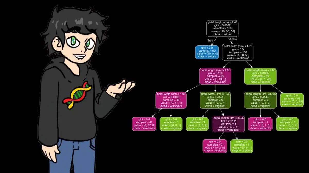
Before feeding data into the classifier, he decided to fully understand how the algorithm works. To do this, he wrote a decision tree from scratch using numpy.
Decision trees work like reasoning games—by asking a series of questions to narrow down the answer.
To illustrate this, he chose a completely different dataset: Titanic.
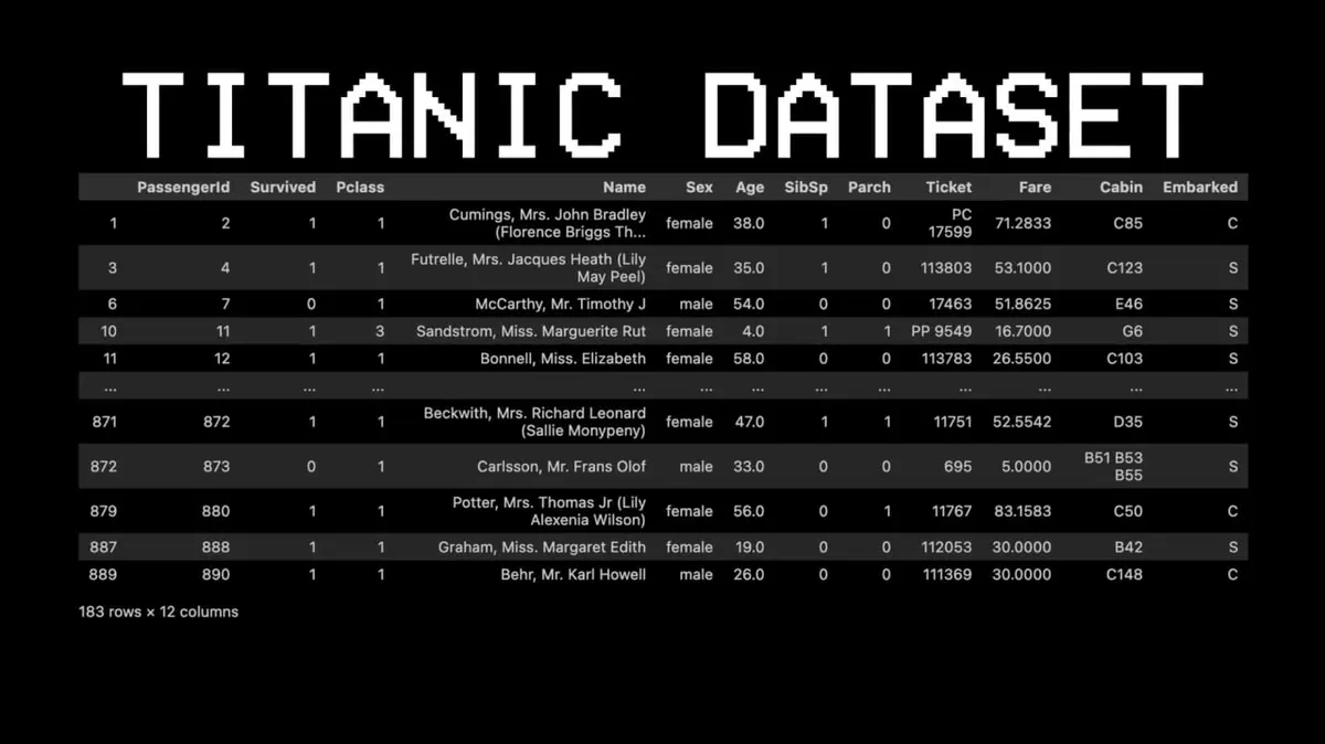
For example: Did passenger #11 survive?
- Question 1: Was he in first class? → Yes.
- Question 2: Was he female? → Yes.
- Predicted outcome: Survived.
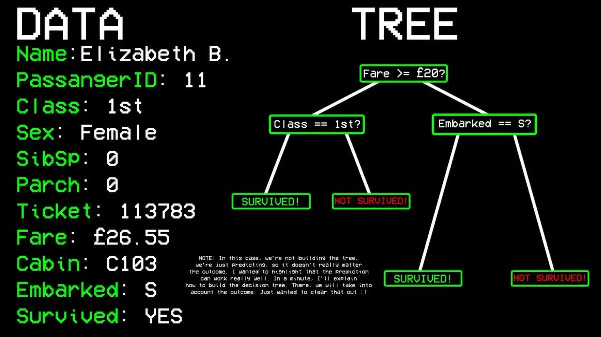
How does the algorithm decide which questions to ask?
It starts with all data, finds the single variable that best separates “survived” and “not survived.” In Titanic data, the answer is passenger class. First-class passengers go one way, others go another.
But even among first-class passengers, some perished, so the split isn’t perfect—there’s “impurity.” The algorithm then looks for the next best split: gender. All female first-class passengers survived, forming a “pure node,” and the branch stops here.
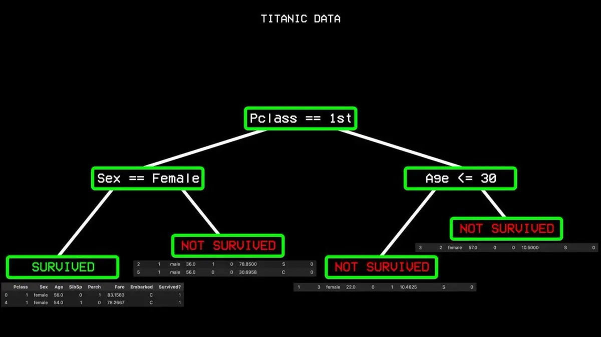
This process repeats until a complete decision tree covering all cases is built.
His numpy version performed well on small datasets, but on 95,000 matches, it was painfully slow. So, during training, he switched to the optimized version in sklearn, which has the same logic but runs much faster.
Step Three: Finding the Key Variables That Decide the Outcome
Before training the model, he plotted all variables against each other in a huge scatterplot matrix (SNS pairplot) to find patterns that distinguish winners from losers.
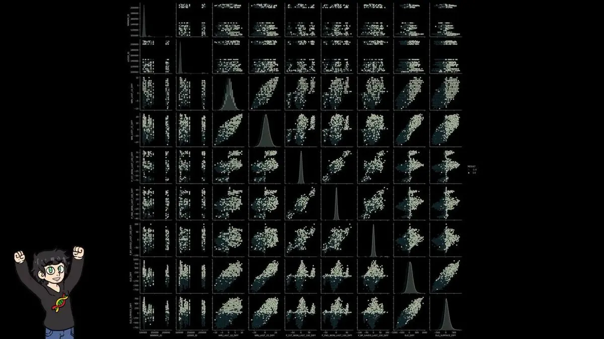
Most features were noise. Player IDs were obviously useless. Win rate differences showed some pattern but weren’t clear enough for reliable classification.
Only one variable stood out: ELO difference (ELO_DIFF).
Scatter plots of ELO_DIFF and ELO_SURFACE_DIFF clearly showed separation between the two classes, far better than any other feature.
This discovery led him to build the core part of the project.
Step Four: Introducing Chess Rating Systems into Tennis
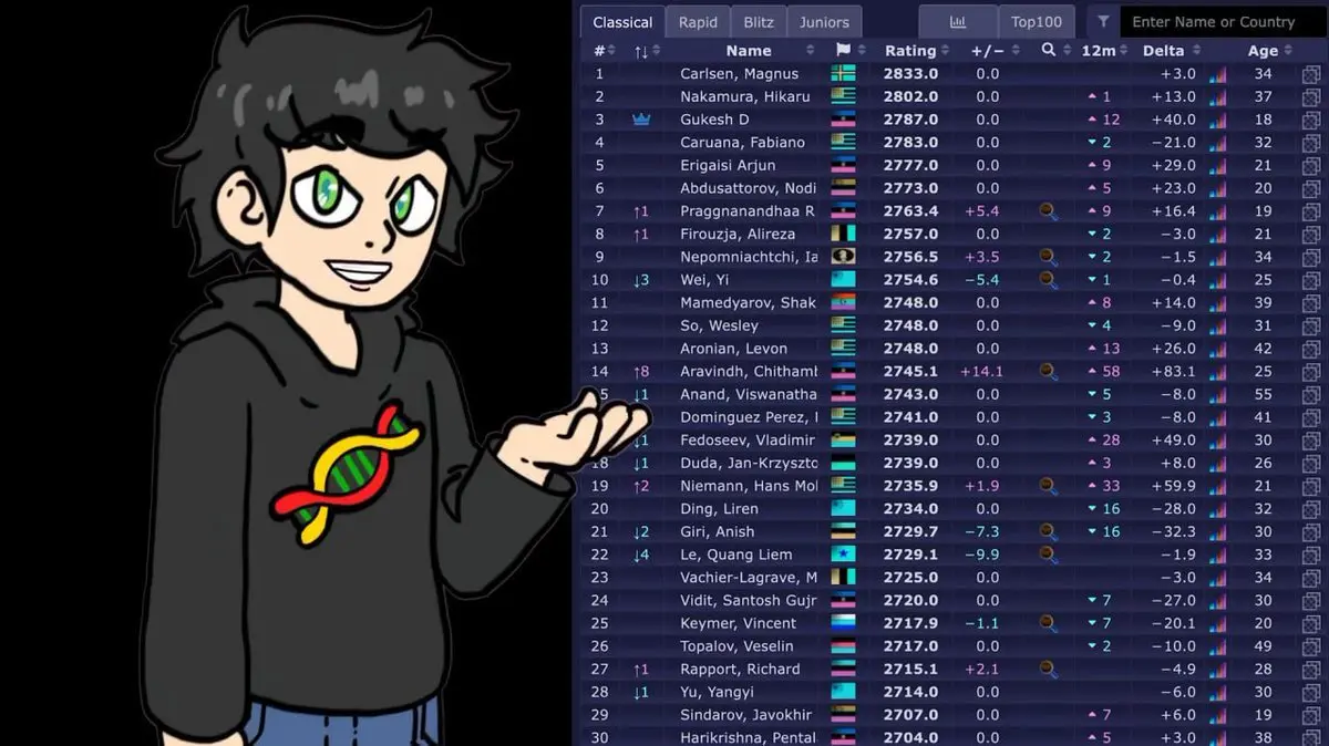
ELO is a method for evaluating players’ skill levels, originally used in chess. The current world number one Magnus Carlsen has a rating of 2833.
He decided to apply this system to tennis:
- Each player starts with a rating of 1500 points
- Winning increases rating; losing decreases it
The key mechanism: the amount of points gained or lost depends on the rating difference with the opponent. Beating a higher-rated player earns more points; losing to a lower-rated player costs more.
He demonstrated this with the 2023 Wimbledon final: Carlos Alcaraz (rating 2063) vs. Novak Djokovic (rating 2120). Alcaraz’s victory increased his rating by 14 points, Djokovic’s decreased by 14.
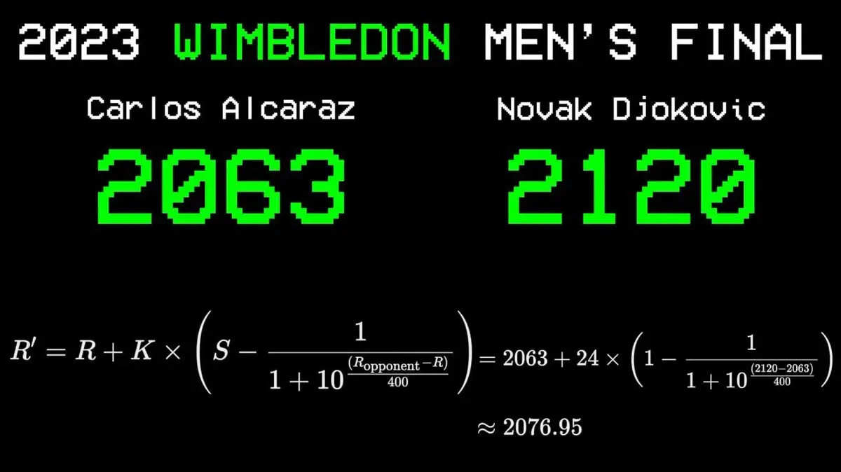
Applying this simple formula across 43 years of data proved to be powerful.
Step Five: Visual Proof of the Big Three’s Dominance
He plotted Federer’s entire career ELO rating as a curve, from debut to retirement, recording every match.
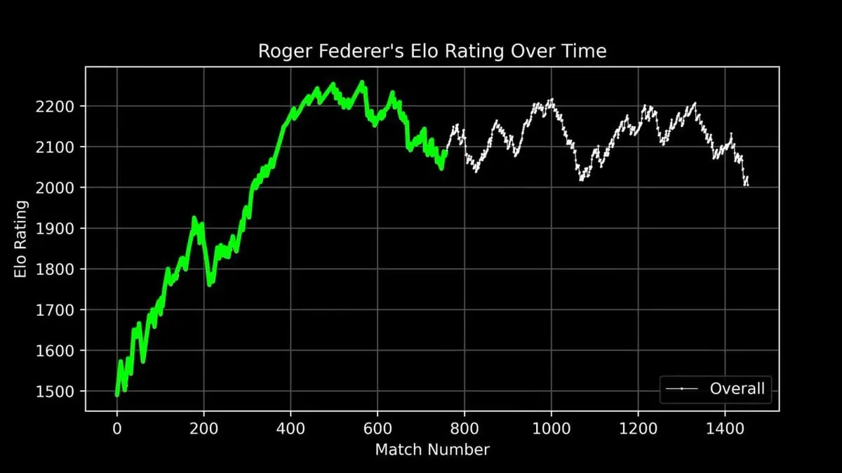
This curve tells a legendary story: rapid rise early on, peak dominance around the 400th match, and fluctuations later in his career.
But what’s truly shocking is when he plotted Federer alongside all ATP players since 1985:
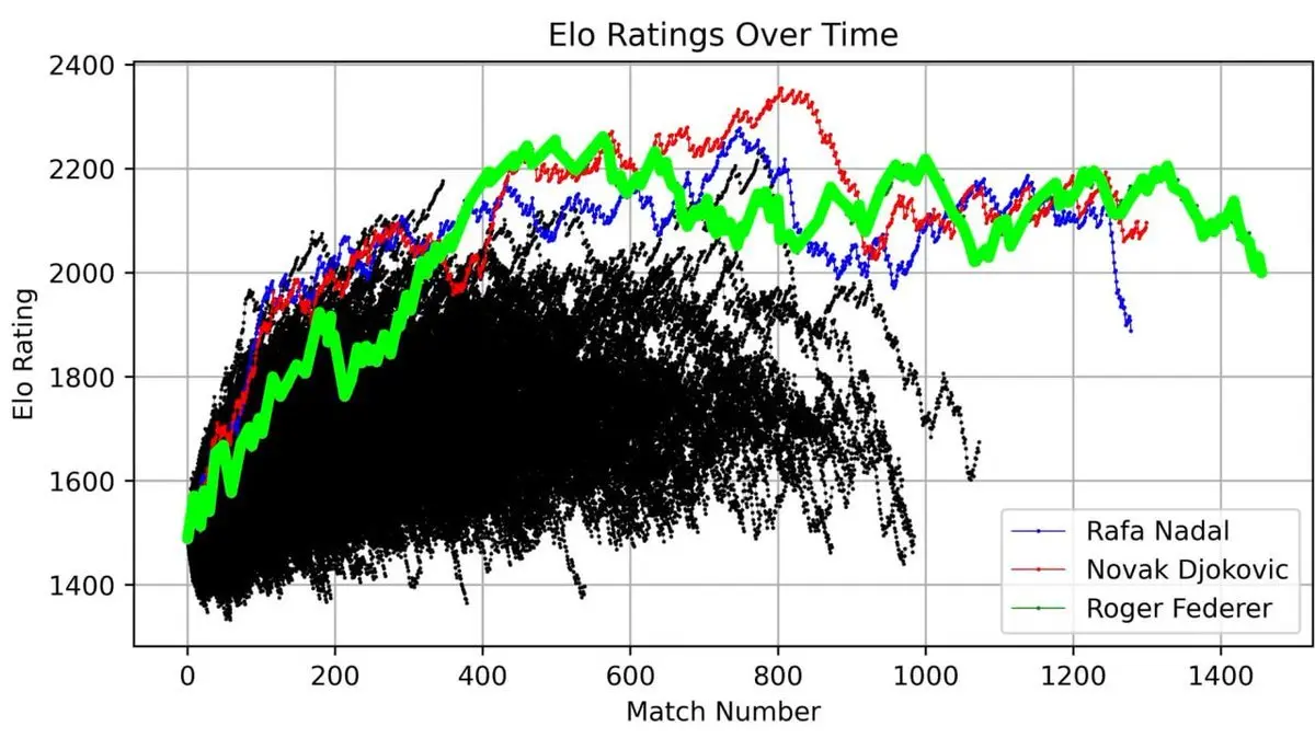
Three lines towered above all others—Federer (green), Nadal (blue), Djokovic (red).
The “Big Three” are not just titles. When visualized with 40 years of data, their dominance is mathematically undeniable.
According to his custom ELO system, the current world number one is Jannik Sinner (2176 points), followed by Djokovic (2096) and Alcaraz (2003).
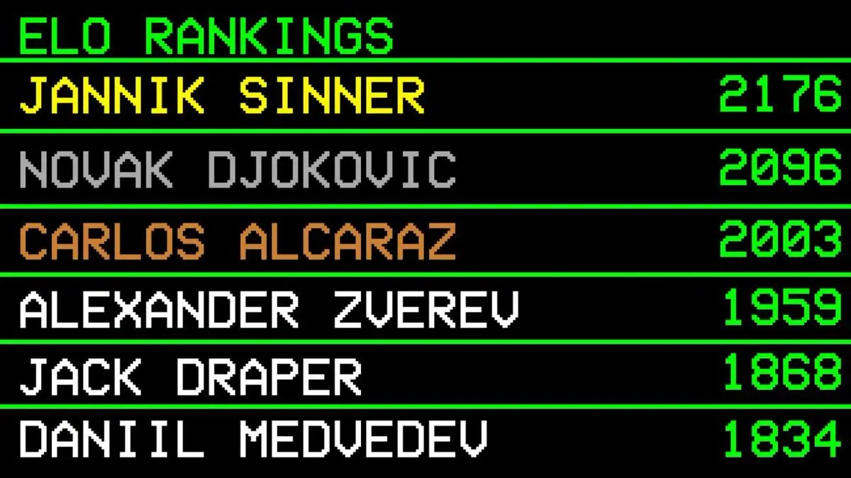
Remembering Sinner’s top ranking is crucial for what follows.
Step Six: Surface as the Variable That Changes Everything
Court surface drastically alters the game:
- Clay: slow, high bounce
- Grass: fast, low bounce
- Hard court: in between
A player who dominates on one surface might struggle on another.
He built separate ELO ratings for each surface: clay, grass, hard court.
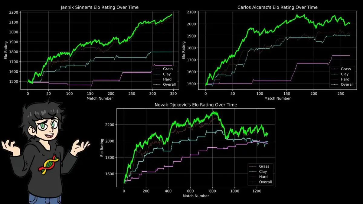
The results confirmed what tennis fans know: Nadal’s peak on clay exceeds Federer’s best on grass, which surpasses Djokovic’s on hard court, and all-time peaks across surfaces.
Nadal’s 14 French Open titles, with 112 wins and only 4 losses, exemplify this.
ELO doesn’t care about narratives or fame; it only processes win-loss records. Its conclusions align perfectly with 40 years of sports news.
Step Seven: Facing the Ceiling
Data ready, ELO system built, he trained classifiers. This process vividly shows the importance of algorithm choice.
Decision tree: 74% accuracy
A single decision tree on the full dataset achieved 74%. Not bad—until you realize that just using ELO difference alone already reaches 72%.
The decision tree added little value on top of his manually crafted rating system.
Random forest: 76% accuracy
The problem with a single tree is “high variance”—it’s overly sensitive to the specific data subset it trained on. The standard solution: random forest—dozens or hundreds of trees trained on different random subsets and features, then vote.
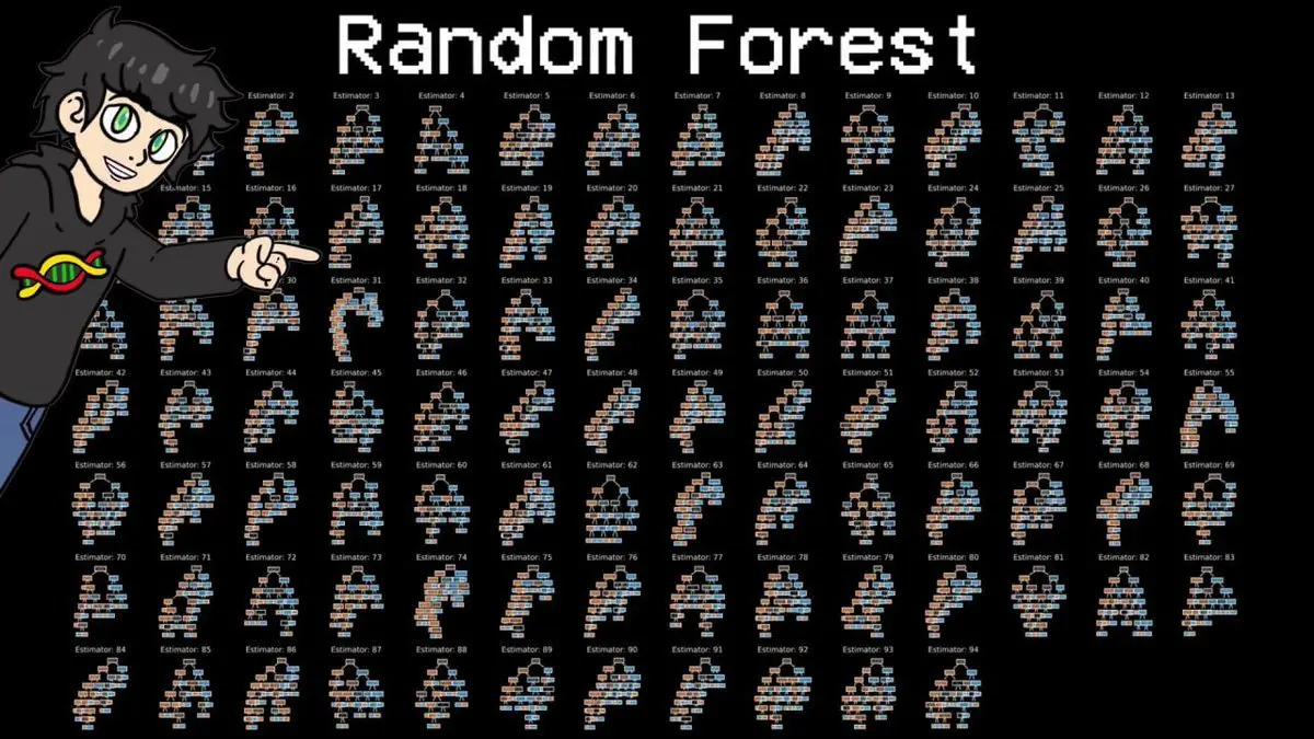
94 diverse decision trees vote on each match.
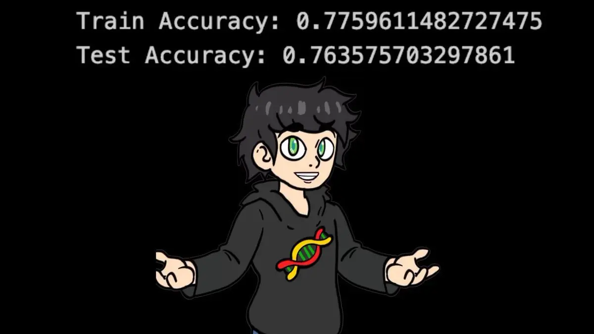
Result: 76%. An improvement, but he hit a ceiling. No matter how he tuned hyperparameters, redesigned features, or tinkered with data, accuracy wouldn’t go beyond 77%.
Step Eight: Breaking Through the Ceiling
Next, he tried XGBoost—what he calls “steroid version of random forest.”
The key difference: random forest builds trees in parallel and averages; XGBoost builds trees sequentially, each correcting the errors of previous ones. It includes regularization to prevent overfitting and keeps each tree small to avoid memorization.
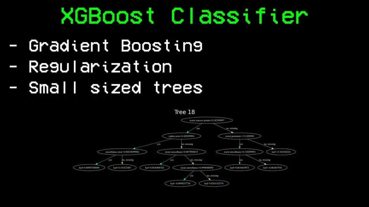
The result: 85% accuracy.
Compared to the 76% ceiling of random forest, this is a huge breakthrough. Same data, same features, only the algorithm changed.
XGBoost also identified the top three features as: ELO difference, surface-specific ELO difference, and overall ELO. This chess-inspired rating system proved to be the strongest predictor among 81 features.
For comparison, he trained a neural network on the same data, achieving 83% accuracy. Good, but still behind XGBoost. On this dataset, tree-based methods outperform.
Step Nine: The Final Showdown—2025 Australian Open
All previous work was based on data up to December 2024.
The 2025 Australian Open, held in January, was completely outside the training set, making it the perfect test: does the model truly understand tennis rules, or just memorize historical patterns?
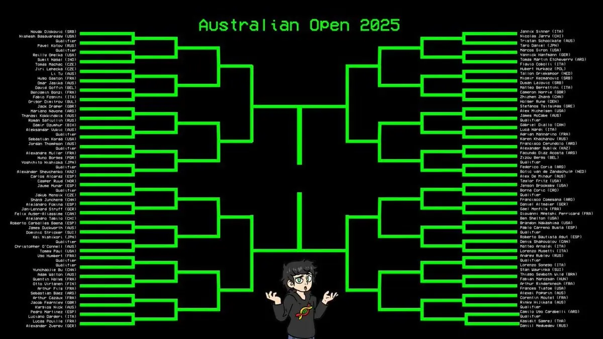
He input the entire tournament bracket into the model to predict each match.
Result: 99 correct predictions out of 116 matches, only 17 errors. Accuracy: 85.3%.
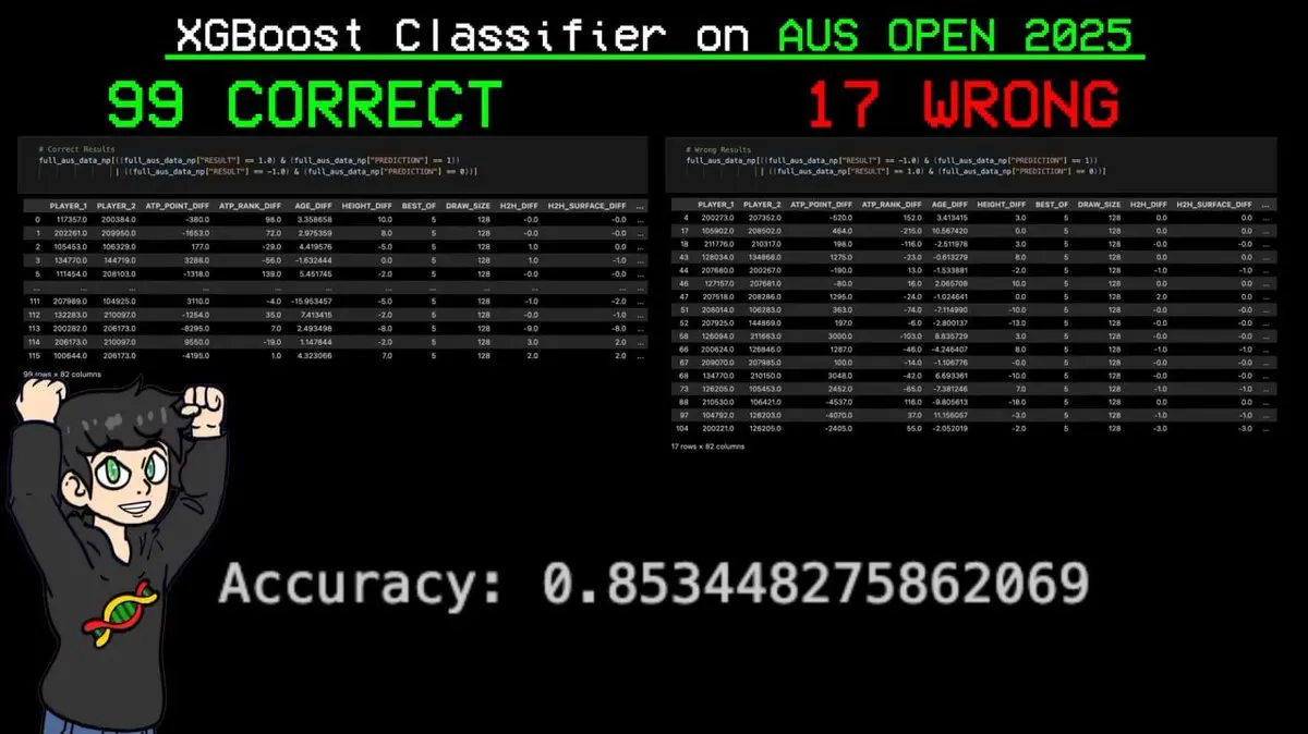
Most importantly, the model accurately predicted Sinner’s every victory throughout the tournament—despite Sinner being the top-ranked player in the ELO system.
Before the first serve, the AI predicted the Grand Slam champion.
Final Words
One person, one laptop, no proprietary data, no expensive infrastructure, no research team—yet built a professional tennis prediction model with 85% accuracy, predicting the Grand Slam winner before the tournament even started.
Tennis data is available on GitHub, fully reproducible.
Creating miracles has never been more within reach.
The real gap isn’t resources, but whether you’re willing to do the work.